Why does your model lose despite its perfect backtest results?

Backtests show that my model makes money, but you find it losing a lot of money when you actually running it!

I suppose every system trader who uses machine learning has such an experience. In this article, I would like to explain one of the reason for this phenomenon by using the mechanism of spurious regression.

(I'm going to use a little bit of arithmetic, but I'll write it down much more clearly)

First, let's consider two unrelated random walks $x_t$ and $y_t$ ($\epsilon$ is white noise).

$$y_t = y_{t-1} + \epsilon_{yt} \\ x_t = x_{t-1} + \epsilon_{xt}$$

Let's try a linear regression of this.

$${\displaystyle y_{t}=\alpha +\beta x_{t}+\epsilon _{t}}$$

Of course, since the two time series are random walks unrelated to each other, you can see that the true value of $\alpha$ and $\beta$ are zero. Let's check this in practice.

Pearson's correlation coefficient$r_{xy}$ is given by the following equation:

$$r_{xy} = \frac{\sum_{t=1}^{T} (x_t - \bar{x})(y_t- \bar{y})}{\sqrt{\sum_{t=1}^{T} (x_t - \bar{x})^2 \sum_{t=1}^{n} (y_t - \bar{y})^2}}$$

Transform it just a little bit:

$$r_{xy} = \frac{\frac{1}{T} \sum_{t=1}^{T} \frac{1}{\sqrt{T}} (x_t - \bar{x})\frac{1}{\sqrt{T}} (y_t - \bar{y})}{\sqrt{\frac{1}{T^2} \sum_{t=1}^{T}\frac{1}{T} (x_t - \bar{x})^2 \sum_{t=1}^{T}\frac{1}{T} (y_t - \bar{y})^2}}$$

Now, those of you who are skilled in probability theory can see from this formula that we can use Donsker's theorem.

Donsker's Theorem.

A time series of cumulative sums of independent identically distributed random variables converges to Brownian motion under some scaling. Namely, Let $X_1,X_2,X_3, .... X_n$ be independent identically distributed random variables with its mean 0 and variance 1,

$$\sqrt{\frac{1}{n}} X_n(r) \rightarrow W(r) (n \rightarrow \infty)$$

We extend this Donsker's theorem by taking integrals on both sides (Continuous Mapping Theorem).

$$\int_0^1 \sqrt{\frac{1}{n}} X_n(r)dr \rightarrow \int_0^1 W(r)dr (n \rightarrow \infty)$$

Now by using the following quations,

$$\int_0^1 x_t(r)dr = \sum_{t=1}^{T} \frac{x_t}{T}$$ $$\bar{x_t}=\sum_{t=1}^{T} \frac{x_t}{T}$$

The numerator of the $r_{xy}$ equation is

$${\frac{1}{T} \sum_{t=1}^{T} \frac{1}{\sqrt{T}} (x_t - \bar{x})\frac{1}{\sqrt{T}} (y_t - \bar{y})}$$ $$\rightarrow \int_0^1 \bigg(W_1(r)dr - \int_0^1 W_1(r)dr \bigg) \bigg(W_2(r)dr - \int_0^1 W_2(r)dr \bigg)dr$$

Also, the denominator is

$$\sqrt{\frac{1}{T^2} \sum_{t=1}^{T}\frac{1}{T} \bigg(x_t - \bar{x}\bigg)^2 \sum_{t=1}^{T}\frac{1}{T} \bigg(y_t - \bar{y}\bigg)^2}$$ $$\rightarrow \sqrt{\int_0^1 \bigg(W_1(r)dr - \int_0^1 W_1(r)dr \bigg)^{2} dr \bigg(W_2(r)dr - \int_0^1 W_2(r)dr \bigg)^2dr}$$

and $T$ has disappeared. This means that the correlation coefficient $r_{xy}$ does not converge to zero. The $F$ test statistic for $\alpha$ and $\beta$ derived from the least squares method also rejects the null hypothesis that $\beta=0$.

What it means?

Depending on the nature of the time series, two completely unrelated series can be shown to be statistically significant. you find this sounds very dangerous.

For example, let's say you have discovered a feature X and have built a model that uses it to predict the price of Bitcoin. First of all, you would statistically analyze whether the feature is really significant or not. However, if the feature is a process with a unit root (unit root process), it will show statistically significant results even if the feature is completely meaningless.

And this is not limited to classical statistical models. Every time series model, whether it be machine learning or a Bayesian model, is based on the assumption of stationarity of the series. Regardless of the mathematical approach, models that ignore the nature of time series will always fail.

Let's try it out

You may feel it just by talking about theory, so let's actually try it out.

Let's generate two random walks using Python and look at the coefficient of determination ($R^2$) derived by the method of least squares (OLS).

import numpy as np
import statsmodels.api as sm
from matplotlib import pyplot as plt
plt.rcParams["figure.figsize"] = (7, 5)
plt.rcParams["figure.facecolor"] = 'grey'

x = np.cumsum(np.random.standard_normal(size=1000000))
y = np.cumsum(np.random.standard_normal(size=1000000))

plt.plot(x)
plt.plot(y)
plt.legend(['x','y'])
plt.show()

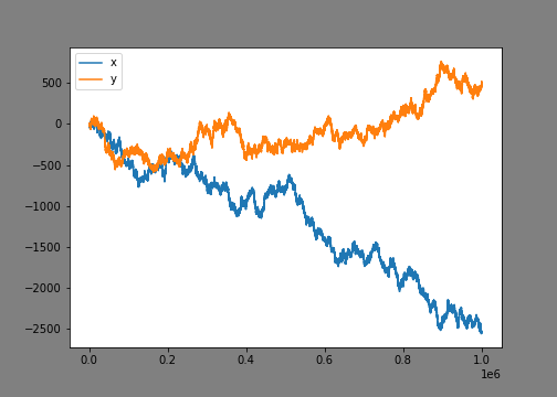
This draws two random walks. At a quick glance, to the human eye, it doesn't look like there's any correlation.。

There are many ways to find the coefficient of determination in Python, but we will use the package statsmodels.

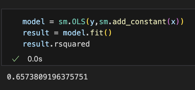
When using the least squares method, the coefficient of determination takes a real number between 0 and 1. Two series that should be uncorrelated show a high correlation of 0.65.

Summary

We have found that even completely meaningless features may show statistical significance depending on the nature of the time series.

Before incorporating a feature into a model, be sure to examine the nature of the data using an ADF test, etc., and properly remove the ineligible features from the model.